5.9 Visualization of unpaired electrons
After a multiconfigurational/multireference calculation is accomplished, people often want to know where the unpaired electron is, or at which atom(s) are unpaired electrons located. 3 approaches are introduced below.
5.9.1 Visualization of natural orbitals
Taking the triangulene molecule as an example
The geometry has been optimized at the UCAM-B3LYP/6-31G(d,p) level. This molecule has a triplet ground state (T0). But firstly, let’s perform the CASSCF calculation of the lowest singlet (S1), which is expected to be of significant biradical/diradical character. The input file of automr (say, triangulene_cc-pVDZ_S.gjf) is
%mem=96GB
%nprocshared=48
#p CASSCF/cc-pVDZ

mokit{FcGVB,Npair=11,GVB_conv=5d-4,LocalM=Boys}

0 1
C       -6.99392200   -0.69965300    0.03089200
C       -6.99037600   -2.08681100    0.00754000
C       -5.79692300   -2.79373800   -0.01900700
C       -4.55293000   -2.11706000   -0.02294700
C       -4.54759300   -0.69024300    0.00094600
C       -5.77962500    0.02901000    0.02825000
C       -3.32798900   -2.80487500   -0.04954900
C       -2.09696100   -2.12716900   -0.05329300
C       -2.08976500   -0.70050100   -0.02943100
C       -3.31558100    0.01410700   -0.00232100
C       -0.85924300   -2.81425700   -0.08011500
C        0.34050600   -2.11749600   -0.08271500
C        0.35636800   -0.73047500   -0.05962300
C       -0.85143000    0.00846700   -0.03273200
C       -3.30942000    1.43300300    0.02142600
C       -4.54239100    2.15073200    0.04875200
C       -5.75083800    1.43372600    0.05151200
C       -0.86802700    1.41341100   -0.00896700
C       -2.07013000    2.14041600    0.01811300
C       -2.09382400    3.55612800    0.04213800
C       -3.29698300    4.24638100    0.06855300
C       -4.50617000    3.56622700    0.07202700
H       -7.93196300   -0.15396700    0.05161000
H       -7.93251100   -2.62540600    0.01006600
H       -5.80270700   -3.87898600   -0.03717500
H       -3.33266200   -3.89097400   -0.06780500
H       -0.86309200   -3.89951400   -0.09839300
H        1.27782500   -2.66405100   -0.10333100
H        1.29927000   -0.19284000   -0.06197400
H       -1.15202100    4.09568800    0.03963300
H       -3.29222900    5.33144200    0.08668400
H       -5.44315500    4.11372400    0.09272200
H        0.07497000    1.95259200   -0.01139400
H       -6.68913500    1.98066500    0.07227600
Keywords in mokit{} are specified to make the GVB SCF not converged to \( \sigma \) - \( \pi \) mixing solution, so that 11 pure C=C \( \pi \) bonding orbitals and 11 pure \( \pi \)* anti-bonding orbitals will be used in CASSCF calculations. Submit this job
automr triangulene_cc-pVDZ_S.gjf >triangulene_cc-pVDZ_S.out 2>&1
This job will take about 5 hours using 48 CPU cores. Since the active space would be (22,22), the CASSCF would automatically be switched to DMRG-CASSCF during calculation. After the job is accomplished, we obtain 3 fch files which includes natural orbtials
triangulene_cc-pVDZ_S_uhf_uno.fch
triangulene_cc-pVDZ_S_uhf_uno_asrot2gvb11_s.fch
triangulene_cc-pVDZ_S_uhf_gvb11_CASSCF_NO.fch
which include UHF natural orbitals (UNOs), GVB NOs, and CASSCF NOs, respectively.
Choose a file, open it using GaussView, click MO Editor, and click Visualize (if it is in grey color and cannot be clicked, it implies that you need to install the Gaussian software). By default, the 72th and 73th NOs are supposed to be highlighted. If they are not, you can click/choose them to be highlighted. Change Isovalue if you want (0.04 will be used in the following figures). Finally, click Update and wait for a few seconds.
Here are the HONO and LUNO of GVB and DMRG-CASSCF calculations, respectively
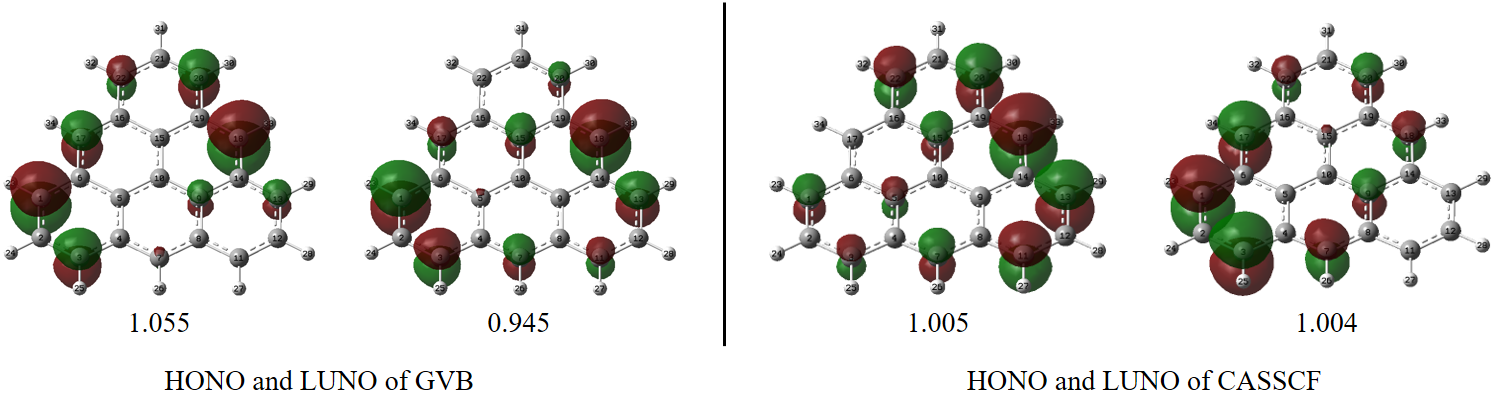
(NOONs are shown below corresponding orbitals)
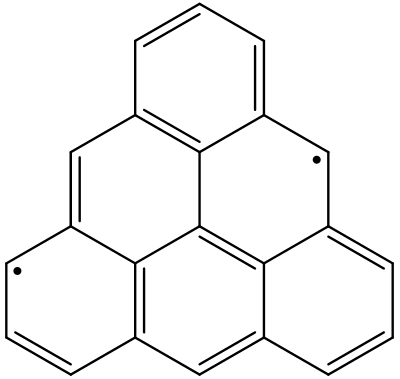
The natural orbital occupation numbers (NOONs) of HONO and LUNO are close to 1.0, which means 1 unpaired electron is occupied in each of these orbitals. It can be seen that these NOs are somewhat delocalized, but mainly with C_1 and C_18 the largest populations. So the following skeletal formula may represent the molecule better
Moreover, the number of unpaired electrons can be found in output
E(GVB) =      -840.26647527 a.u.
----------------------- Radical index -----------------------
biradical character   (2c^2) y0=  0.945
tetraradical character(2c^2) y1=  0.038
Yamaguchi's unpaired electrons  (sum_n n(2-n)      ):  3.086
Head-Gordon's unpaired electrons(sum_n min(n,(2-n))):  2.445
Head-Gordon's unpaired electrons(sum_n (n(2-n))^2  ):  2.051
-------------------------------------------------------------
...
E(CASSCF) =      -840.43136870 a.u.
----------------------- Radical index -----------------------
biradical character   (2c^2) y0=  1.004
tetraradical character(2c^2) y1=  0.129
Yamaguchi's unpaired electrons  (sum_n n(2-n)      ):  5.015
Head-Gordon's unpaired electrons(sum_n min(n,(2-n))):  3.572
Head-Gordon's unpaired electrons(sum_n (n(2-n))^2  ):  2.531
-------------------------------------------------------------
The number of unpaired electrons are calculated based on all NOs, so they will be slightly larger than 2 (the definition sum_n (n(2-n))^2 is recommended). Anyway, we know that there exists 2 unpaired electrons for the S1 state of this molecule.
If you think DMRG-CASSCF calculation is too expensive, you can perform only the GVB calculation, and use GVB NOs in the *_s.fch file to demonstrate unpaired electrons or diradical characters.
Note that these techniques/tricks can, of course, also be applied to the analysis of single reference calculations. For example, assuming we want to find the open-shell singlet excited state of the ethene molecule using RKS-based TDDFT. Here is the ethene.gjf file
%chk=ethene.chk
%mem=16GB
%nprocshared=8
#p PBE1PBE/cc-pVDZ TD(nstates=10) nosymm int=nobasistransform density

title

0 1
 C                 -1.76890146   -0.14978602    0.00000000
 H                 -1.23573772   -1.07749094    0.00000000
 H                 -2.83890146   -0.14978602    0.00000000
 C                 -1.09362716    1.02519128    0.00000000
 H                 -1.62679090    1.95289620    0.00000000
 H                 -0.02362716    1.02519128    0.00000000


--Link1--
%chk=ethene.chk
%mem=16GB
%nprocshared=8
#p PBE1PBE chkbasis nosymm int=nobasistransform guess(read,only,save,NaturalOrbitals) geom=allcheck
Once the the Gaussian job is accomplished, you can find the S1 state is mainly contributed by 8->9 excitation
 Excited State   1:      Singlet-?Sym    7.9680 eV  155.60 nm  f=0.3635  <S**2>=0.000
       8 ->  9         0.70368
       8 <-  9        -0.10343
Since TDDFT only takes one-electron excitations into consideration and RKS-based TDDFT in Gaussian is a spin-adapted method, 8->9 excitation stands for the linear combination of two Slater determinants sqrt(2)/2 (8a9b - 8b9a), which is open-shell singlet.
We can double check via TDDFT NOs. Run
formchk ethene.chk ethene.fch
Natural orbitals of the S1 state are kept in ethene.fch. NOs with occupation numbers significantly deviate from 2.0/0.0 are
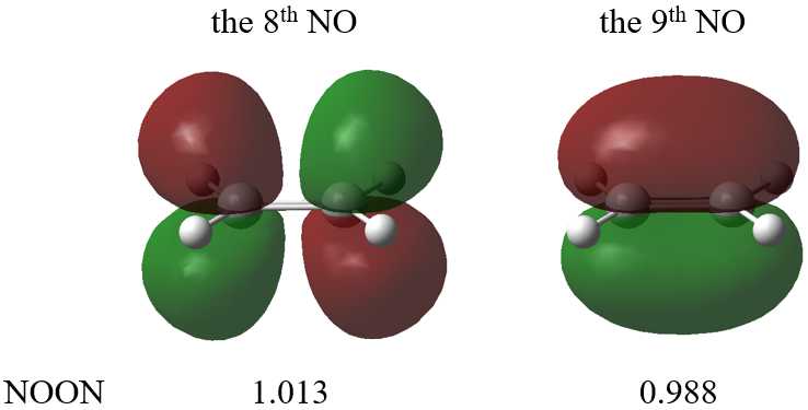
which means that the C-C pi/pi* orbital has one unpaired electron, respectively. Whether using unrelaxed or relaxed density usually does not matter here. See Section 5.9.3 below for unpaired electrons and unpaired electron density.
5.9.2 Visualization of localized active orbitals
You might notice that for the example shown above, the CASSCF occupation number of HONO happens to be almost equal to that of LUNO. It can be viewed as degeneracy in occupation numbers. So we can perform orbital localization upon these 2 NOs without changing their occupation numbers. Start Python and run
from mokit.lib.gaussian import loc
loc(fchname='triangulene_cc-pVDZ_S_uhf_gvb11_CASSCF_NO.fch',idx=range(71,73))
Then a file named triangulene_cc-pVDZ_S_uhf_gvb11_CASSCF_NO_LMO.fch is obtained. These two active orbitals will become a little more localized.
This trick can also be applied to high-spin triplet GVB or CASSCF calculations, in which there will be (at least) two unpaired alpha electrons in GVB or CASSCF NOs. Whenever singly occupied orbitals are delocalized, orbital localization will do much help.
Note that if you apply this trick to NOs which are not degenerate in occupation numbers, their occupation numbers will no longer exist, and only occupation number expectation values exist (i.e. the occupation number matrix becomes not diagonal).
5.9.3 Visualization of unpaired electron density
In unrestricted DFT (UDFT) calculations, people often visualize the spin density to find where the unpaired electrons are. In multiconfigurational methods, the unpaired electron density (also called odd electron density) is often used to show the spatial distribution of unpaired electrons. Using the CASSCF NOs of the S1 state as an example, start Python and run
from mokit.lib.wfn_analysis import calc_unpaired_from_fch
calc_unpaired_from_fch(fchname='triangulene_cc-pVDZ_S_uhf_gvb11_CASSCF_NO.fch',wfn_type=3,gen_dm=True)
This will generate the unpaired electron density stored in triangulene_cc-pVDZ_S_uhf_gvb11_CASSCF_NO_unpaired.fch. There are various ways to visualize the unpaired electron density:
(1) Visualizing via GaussView
Run the following command in Shell
cubegen 48 fdensity triangulene_cc-pVDZ_S_uhf_gvb11_CASSCF_NO_unpaired.fch triangulene_unpaired.cub -3 h
which uses 48 CPU cores to generate the cube file. Note here the fdensity cannot be replaced by density=SCF.
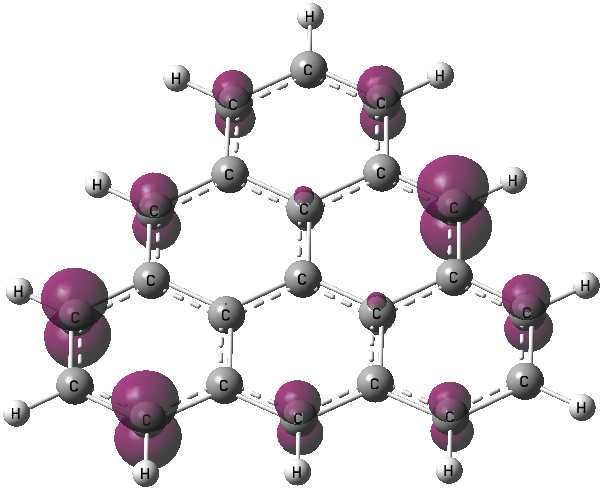
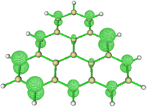
Open the file triangulene_unpaired.cub with GaussView, click Results on the panel, click Surfaces/Contours, change the value of Density = to 0.01 a.u., click Surface Actions and finally click New surface. The plot would be like
(2) Visualizing via Multiwfn
Start Multiwfn and load the file triangulene_cc-pVDZ_S_uhf_gvb11_CASSCF_NO_unpaired.fch, then type
200
16
SCF
y
0
5
1
3
-1
The key idea is to make Multiwfn read the Total SCF Density section in .fch file and generate corresponding cubes. Note that the procedure above (i.e. integers input interactively) may be slightly different for different versions of Multiwfn, you should pay attention to the information/hints shown in the Multiwfn cmd window. Finally, change the Isosurface value to 0.01 a.u. and the plot would be like
Of course, you can use also Multiwfn + VMD to get even better plots.
Note that the unpaired electrons as well as density can, of course, also be applied to the analysis of single reference calculations (MP2, CCSD, TDDFT, etc). Taking the S1 natural orbtial file ethene.fch as an example, running the following Python script
from mokit.lib.wfn_analysis import calc_unpaired_from_fch
calc_unpaired_from_fch(fchname='ethene.fch',wfn_type=3,gen_dm=True)
The number of unpaired electrons are printed on the screen
----------------------- Radical index -----------------------
biradical character y0 = n_LUNO =  0.988
tetraradical character y1 = n_{LUNO+1} =  0.021
Yamaguchi's unpaired electrons  (sum_n n(2-n)      ):  2.169
Head-Gordon's unpaired electrons(sum_n min(n,(2-n))):  2.060
Head-Gordon's unpaired electrons(sum_n (n(2-n))^2  ):  2.004
-------------------------------------------------------------
where an open-shell singlet species is supposed to have about 2.0 unpaired electrons. Besides, the file ethene_unpaired.fch is generated and the unpaired electron density is located on two C atoms
